Jensen’s Inequality, Estimation Bias, and Innovation Investing
January 2022
When computation of a non-linear function relies on an uncertain parameter, then symmetric lower or higher outcomes of the parameter compared to its expected value will generate asymmetric effects on the function’s output. This means that if we restrict ourselves to the probability-weighted average of a parameter — i.e. we solve the function of the expectation — we will get a very different result than if we incorporate the (average-preserving) width of its probability distribution — i.e. we solve the expectation of the function.
We will explore important implications of this statistical inequality on corporate finance and portfolio management, where non-linearity in the form of convexity is often hidden in plain sight. For example, a DCF-generated enterprise value is convex in our assumption of the terminal growth rate, such that if we treat the growth rate as uncertain and simply increase its possible range, we are left with a more valuable company. Theoretically, this logic is at odds with the inference methodology typically advanced in finance textbooks, where we make a stochastic estimate conditioned on a fixed ‘true’ mean; practically, it explains why Elon Musk can drive up the stock price of Tesla by promising a network of robotaxis. We will also try to build some pattern recognition around how parameter uncertainty shapes narratives common to innovation investing, where small likelihood of zero to one — to adopt Peter Thiel’s rhetoric — compensates investors for large likelihood of zero to zero. The overarching goal of this note is to demonstrate that uncertainty in the context of investment valuation, when properly treated as a feature and not a bug, can turn traditional finance intuition on its head.
Overview
Jensen’s inequality states that the convex transformation of a mean is less than or equal to the mean applied after a convex transformation1— formally, f(E(X) ≤ E(f(X) — with the opposite true for a concave transformation. Take for example f(X)=X2, where, at equal likelihood, X(Ω) = { 2, 3, 4 }. The expected value of “X” is 3, which when squared equals 9. The expectation of the function, on the other hand, is (22+32+42)/3=~10. The resultant difference of ~1 is called the Jensen gap. If instead we widen the assumed uniform distribution to X(Ω) = { 1, 3, 5 }, thus maintaining the same expected value of “X”, then the Jensen gap grows to ~3, and for X(Ω) = { 0, 3, 6 }, it grows to ~6. As a result, non-linearity forces us to think carefully about the probability distribution that best describes the uncertainty of X(Ω), since it divorces exposure to a parameter from expected outcome of the parameter.
Within finance, options pricing is a straightforward application of this concept; an out-of-the-money option commands a non-zero premium. In fact, within equity derivatives markets, spreads on variance swaps versus volatility swaps on equity indexes like the S&P 500 come very close to a traded manifestation of the Jensen gap. However, the idea for this note came about due to concealed convexity embedded in valuation functions popularly applied in corporate finance and portfolio management. Here Jensen’s inequality tends to uncover the important positive influence of parameter uncertainty of inputs such as mean earnings growth rates, margins, cost of capital, and period returns on the estimation of investment values. This uncertainty is frequently neglected by the finance community when practitioners effectively treat such parameters as deterministic, sensitizing valuation outputs against parameter point estimates but not against width of the underlying distributions that are centered on these point estimates.
I will investigate two types of non-linear estimation where second-order thinking on key parameters can conceptually justify investment decisions that on the surface may appear irrational. First we will focus on the dot-com technology bubble and explore what levels of uncertainty in future ROE of Nasdaq stocks can solve for peak Nasdaq valuations observed in March 2000, despite sticking to reasonable average future ROE, as well as how outsized R&D spending in the late 1990s contributed to this uncertainty. We will also briefly assess how accretion of equity value under earnings growth uncertainty is mechanically boosted by the current divergence of real GPD growth and real yields (adding an important extra layer to the commonly discussed, but seemingly underestimated, vulnerability of technology stocks to higher interest rates). Second we will explore why the textbook recommendation that we should make investment decisions based on unbiased long-term mean returns encounters problems under Jensen’s inequality. An approach per classical logic infers a stochastic mean return estimate while assuming there exists a fixed true mean return. However, an approach per more relevant investor logic infers an uncertain true mean outcome drawn from a distribution that is centered on a fixed mean return estimate. Given cumulative return is a convex function of mean return, we will see why parameter uncertainty can allow investor logic to rationally pursue investments that classical logic rejects, potentially even including opportunities with negative short-term risk premia or alpha. What unites these two investigations is that they both demonstrate the explanatory power of uncertainty over investment value when a parameter outcome — like mean earnings growth or mean return — can compound over time.
Given these two examples, where compounding relates a symmetric parameter distribution to a positively skewed investment value distribution, we will close by taking a closer look at innovation investing, where underlying parameter distributions themselves are also positively skewed. Disruptive technologies are unlikely to gain critical mass but promise monopolistic profits if they do succeed. Jensen’s inequality implies that here we are mostly paying for uncertainty rather than average expectation of the mean technology adoption rate. Mathematically, the center of this distribution can largely become noise — instead, information resides in the right tail of technology adoption and, with a boosted effect, valuation outcomes. Hence equity investments in disruptive technologies feature super high variability to the upside, while losses are bounded by design at committed capital to the downside. We will assess why this makes a related epistemological problem — that we cannot observe probability distributions, only realizations — more potent and conceptualizes the venture capitalist’s job as avoiding thin-tailed business models. Finally, I will caution that not everyone can afford to de-prioritize median outcomes, and propose that a corollary to this logic comes to the defense of an asset class that the modern, technology-forward yet inflation-wary investor has developed quite the distaste for: fixed income.
Convexity in Investments Example #1: Intrinsic Value via Future Mean Earnings Growth
One of the most common case studies on irrationality in the history of financial markets is the dot-com bubble that burst in early 2000. In their 2004 paper “Was there a Nasdaq bubble in the late 1990s?”, authors Pastor and Veronesi use as motivation Garber’s challenge that “bubble characterizations should be a last resort because they are non-explanations of events”2. In other words, calling the tech boom a bubble means we do not understand why it happened. In search for an explanation, Pastor and Veronesi focus on the link between uncertainty about a firm’s average future earnings growth rate and the firm’s equity valuation; ceteris paribus, a rich earnings multiple need not be driven by expectation of a high future growth rate, but can instead be justified by a sufficiently wide underlying distribution from which the growth rate is drawn. Hence the core idea is that “a firm with some probability of failing (a very low “g”) and some probability of becoming the next Microsoft (a very high “g”) is very valuable”2.
To see why Jensen’s inequality is commonly at work in equity valuations, we don’t need to look further than the traditional gordon growth model. Given P=D/(r-g), where “P” is the stock price, “D” is the next period dividend, “r” is the discount rate, and “g’ is the mean future growth rate, then “P” is a convex function of “g”. As a result of this non-linearity, the distribution of “g” drives expectation of the value function: E(D/(r-g)) ≥ D/(r-E(g)). Similarly, in a DCF as constructed in corporate finance practice, when we multiply the year 5 free cash flow present value by (1+g)/(r-g) to generate a terminal value, then both the terminal growth rate and prior period compounded growth rates implicit in year 1-5 free cash flow projections trigger Jensen’s inequality in our estimation of firm enterprise value. As a result, we can solve for the implied uncertainty of average growth rates that computes observed tech bubble stock prices, similar to how we can solve for Black-Scholes implied volatility of stock prices that computes observed market option prices.
In the paper, the authors tackle the issue from a slightly different angle; since technology stocks tend to not pay dividends, they apply the ‘residual income’ model, a popular alternative to the DCF where terminal value tends to account for a lower portion of total projected value. Here market equity equals book equity plus the present value of abnormal earnings. Future abnormal earnings equal net income minus an equity charge based on period book value times cost of equity, and are separately discounted at the cost of equity. Hence a future period is only accretive to a firm’s present value if the period’s ROE exceeds its cost of equity.
In their computations, the authors isolate excess ROE as the difference between Nasdaq firms and NYSE/Amex firms (representing ‘new’ and ‘old’ economies, respectively), layered on top of a mean-reverting process across business cycles for ‘old’ economy profitability. They then subject excess ROE to the uncertainty of a normal distribution. Given future book value compounds at the rate of abnormal earnings, the P/B ratio is a convex function of average future excess profitability. Jensens’ inequality thus takes effect; P/B of the expectation of excess ROE is less than the expectation of P/B under excess ROE drawn from a normal distribution. For example, the authors’ model (of which I have admittedly only given a simplistic account) converts a market-wide equity premium of 3%, Nasdaq excess ROE of 3%, and expectation of Nasdaq abnormal profits for 20 years into both a Nasdaq P/B of 7.4x under an uncertain mean excess ROE with a standard deviation of 3% and a Nasdaq P/B of 4.9x when mean excess ROE is fixed (~50% incremental value from the Jensen gap!). Please also note that per the authors’ calibration, Nasdaq abnormal earnings are discounted based on a required excess return of more than twice the market-wide equity premium.
The table below shows the surprisingly low outputs of % implied excess ROE standard deviation that match the Nasdaq’s observed P/B ratio of 8.55x on March 10th, 2000 — the price peak of the bubble:
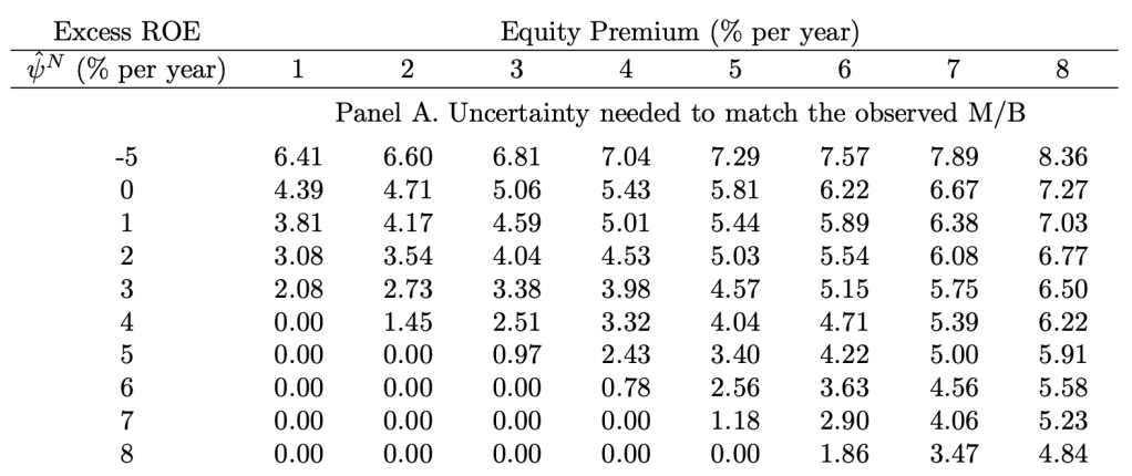
Image source: Ľuboš Pástor, Pietro Veronesi, “Was there a Nasdaq bubble in the late 1990s?”, Journal of Financial Economics, Volume 81, Issue 1, 2006, Pages 61-100, ISSN 0304-405X, https://doi.org/10.1016/j.jfineco.2005.05.009.
Given the current profitability spread in March 2000 was ~9% in favor of NYSE/Amex firms, a positive excess ROE for the Nasdaq may seem far-fetched. But the silver lining of the tech bubble was that it also constituted a ‘productive’ bubble, due to incredibly high associated R&D spending. In the words of Warburg Pincus’ Bill Janeway, the dot-com bubble “both accelerated the build-out of the physical internet and funded the first wave of quasi-Darwinian exploration of this new economic space in search of commercially relevant and financially sustainable ventures”3. Between 1994 and 2004, the ratio of privately financed industrial R&D to GPD rose from 1.4% to 1.9% in the U.S., virtually fully accounted for by companies that had been publicly traded for less than 15 years4. This was financed through massive capital inflows from external equity financing, as commercial opportunity sets suddenly enabled by the internet captured investors’ imagination.
We also have some empirical evidence of investors rapidly changing their mind in a way that points to greater earnings growth uncertainty during this period; average monthly volatility in the year 2000 was 47%, dispersion of profitability across Nasdaq stocks increased, and stock price reactions to earnings announcements were unusually strong2. As technology investors paid up for small probabilities of gigantic future excess profitability, prospectively unlocked by outsized R&D, they also became highly sensitive to new information that marginally revealed accuracy of these probabilities. Jensen’s inequality hence helps us reconcile mathematically why explanatory power over dot-com bubble stock prices seems to have resided in the tails of earnings growth distributions. Investors were likely still irrationally high in the mean of their parameter distributions, but there also were real reasons for and value generated by the width of these distributions.
The mechanics of the positive effect of earnings growth uncertainty on stock prices are particularly important in the context of the Federal Reserve’s continued market intervention in pursuit of loose financial conditions. At a lower risk-free rate or equity risk premium and hence a lower discount rate, more of a firm’s value comes from future earnings, and because of the aforementioned convexity in multi-period compounding, future earnings are more affected by earnings growth uncertainty. As an extension of this logic, we saw terminal value calculations under the gordon growth model are convex functions of the spread between discount rate and growth rate (given denominator “r-g”). As a result, across residual income, DCF, and DDM models, ceteris paribus and for a given level of uncertainty in growth, the Jensen gap is larger when the discount rate falls or the growth rate rises. This implies that the downward pressure of central bank quantitative easing on interest rates — which started after the great financial crisis in 2008 and exploded during the COVID pandemic — has made parameter uncertainty in equity valuations even more potent.
Particularly in 2021 we saw a remarkable divergence in the U.S. between real growth at one of the highest readings since World War II and real yields at all-time lows5. Historically, risk-free rates used to be an approximation of GDP growth (in turn conventionally a proxy for the terminal growth assumptions), but intervention by the Federal Reserve has effectively turned the GDP growth rate into a ceiling for the risk-free rate. This adds another layer to the vulnerability of technology stocks to higher interest rates; when yields normalize relative to growth, we need to worry not only about impairment of terminal value (which typically comprises a large proportion of their total value, given delayed profitability of new technologies) due to higher discounting, but also about impairment of the incremental valuation benefit from earnings growth uncertainty via Jensen’s inequality.


Image source: https://www.blackrock.com/us/individual/insights/beach-ball-investment-pool
Convexity in Investments Example #2: Extrinsic Value via Future Mean Return
Next we will move on to a more theoretical investigation of the role of parameter uncertainty in investment decisions. We will evaluate the way that future mean returns generically translate into cumulative performance. The focus here is on the uncertainty of mean returns, which should not be confused with the standard deviation (i.e. volatility) of returns. Standard deviation reflects variability of per-period returns as they stochastically fall above or below their mean over time, thus preserving the center of the return distribution. Here we are taking for granted ‘irreducible noise’ due to economic uncertainty as measured by standard deviation, and are concerned instead whether the center of the distribution itself should also be treated as noisy. The distinction is consequential under Jensen’s inequality because cumulative investment performance (and hence investment value) across multiple periods is a convex function of mean investment return. Just like in the aforementioned corporate finance examples, the underlying and inescapable force responsible for this non-linearity is compounding. If we are offered a security that compounds at an unknown annual mean return, then we could pursue or reject the opportunity depending on whether we (1) condition ourselves on the true value of mean return under an uncertain estimate or (2) condition ourselves on the mean return estimate under an uncertain truth. We will explore why Jensen’s inequality compels the second (Bayesian-inspired) approach to produce a materially higher investment valuation forecast than the first (classical-inspired) approach.
Generally speaking, textbook finance assumes an investment has one ‘true’ future mean return — but in the context of a time series, how do we even think about a ‘mean’? At the outset, the choice is typically between the arithmetic mean, meaning a simple average of per-period returns, and the geometric mean, meaning a CAGR that relates starting wealth to ending wealth. Under volatile returns, geometric means are always lower than arithmetic means — for example $100*(1-10%)*(1+30%) < $100*((1+10%)2). This is informally known as the ‘volatility tax’ and explains Buffett’s number one rule: ‘don’t lose money’. However, the concept is slightly misleading; compounding of volatility skews the distribution of returns in a way that reduces its median (geometric mean) without actually changing its expectation (arithmetic mean). Higher return volatility over multiple periods implies most likely we’ll end up with less money, but there is now also a still small but marginally higher chance we’ll end up with a lot more money. Such a right tail reflects potential for explosive upward paths when variability happens to compound to the upside. In lognormal distributions, the arithmetic mean exceeds the geometric mean by half the return variance.
If we know the true future arithmetic mean return, then compounding at this rate will produce an unbiased estimate of cumulative return6. The problem is that in practice we don’t know true mean return and instead need to make an uncertain estimate from a historical data series. With the aim to avoid estimation errors, should we use arithmetic or geometric returns? This has been the subject of much debate. In their 2002 paper “Geometric or Arithmetic Mean: A Reconsideration”, Jacquier, Kane, and Marcus argue that we should use neither! Historical arithmetic means are biased upwards under Jensen’s inequality because a positive error in compounded mean return would add more forecasted wealth than a negative error would subtract wealth; symmetric errors thus have asymmetric effects. Meanwhile historical geometric means are biased downwards when the investment horizon is shorter than the sample estimation period. As a result, Jacquier et al. recommend using a weighted average of arithmetic and geometric means to produce an unbiased estimate, based on the ratio of investment horizon to sample estimation period6.
Textbook finance thus teaches us that investment decisions should be made according to unbiased estimates of long-term mean returns. However, in their 2010 paper “Jensen’s Inequality, Parameter Uncertainty, and Multi-Period Investment”, authors Grinblatt and Linnainmaa (I was fortunate to take one of his classes during my undergraduate studies at the University of Chicago) refute this view. They show that, if instead of an uncertain estimate under a single true mean return, we reframe the problem as an uncertain draw from a true mean distribution that is centered on the estimated mean, then “any criterion…(based on) an unbiased estimate of a risky investment’s future value rejects too many good projects”7. As a basis for their argument, they contrast the classical approach of a ‘statistician’ (e.g. by Jacquier et al.) with the quasi-Bayesian approach of an ‘investor’. Both statistician and investor come up with an estimate ‘m’ of mean return ‘μ’, but “the targets they forecast differ…due to Jensen’s inequality and differences in the way they form conditional distributions”.
On the one hand, the statistician treats truth as fixed with the estimate stochastic. Since the statistician conditions on a true value of ‘μ’, she adjusts arithmetic E((1+m)2) downwards for variance of ‘m’ (or instead replaces ‘m’ with a lower weighted average of geometric and arithmetic return) to cleanse its well-known upward bias. The statistician’s objective is to avoid being too high or low across multiple independent forecasts. On the other hand, the investor treats the estimate as fixed with the truth one of many possible outcomes. Since the investor conditions on ‘m’, she adjusts arithmetic (1+m)2 upwards for variance of ‘μ’. Here the investor is focused on the distribution from which the one true outcome of ‘μ’ is drawn. As a result of these different inference methodologies, “one believes that (1 + m)2 underestimates the multi-period future value and the other believes it is an overestimate”. These estimation differences cannot exit in a single-period or linear value function setting. But in a multi-period non-linear setting, where single-period mean returns can compound, “both the statistician and the investor make perfectly rational, but different long-term return forecasts”, as they respectively target V(μ) and E(V(μ)):
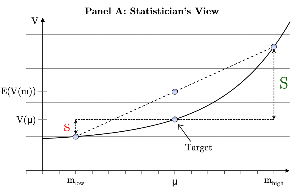

Image source: Grinblatt, Mark and Linnainmaa, Juhani T., Jensen’s Inequality, Parameter Uncertainty, and Multi-Period Investment (October 30, 2010). Chicago Booth Research Paper No. 10-22, CRSP Working Paper, https://ssrn.com/abstract=1629189
When overlaying utility functions, the authors make a surprising discovery: for an investor with sufficiently low risk-aversion (below log utility) under parameter uncertainty, the positive effect of a higher mean dominates the negative effect of higher variance. For such an investor, it may consequently be rational to pursue investments with negative per-period risk premia (i.e. estimated mean return that is lower than the risk-free return). Under similar logic, circumstantially it can make sense to combine passive holdings with active holdings that have negative instantaneous alpha, if uncertainty of alpha and/or horizon length are sufficiently large.
Conclusion: Innovation Investing Through a Probabilistic Lens
Throughout the above sections, we have taken an in-depth look at the way that symmetric uncertainty around true parameter values translates into positive skew in the distribution of modeled investment value. But when we make investments in disruptive technologies, then the underlying parameter distribution — whether in financial terms, such as mean earnings growth, or in operational terms, such as mean technology adoption growth — will frequently exhibit positive skew itself as well. Here the far right tail of a parameter, which under Jensen’s inequality has significant explanatory power over fair value of the investment, tends almost by definition to be a subject of creativity and imagination, rather than of sober, quantitative analysis: at an extreme of topical examples, Tesla running a robotaxi network, or Bitcoin globally replacing fiat currencies. The associated epistemological problem — that we cannot observe probability distributions, only realizations — is more powerful under such thick tails. In his opposition to the commonly used central limit theorem, Nicholas Taleb formulates this as the ‘masquerade problem’8; we cannot rule out thick tails, but we can rule out thin tails. This conceptualizes the challenge of venture capitalists to pick winners as an exercise in avoiding thin-tailed business models. Peter Thiel’s advice for startups to avoid competition and build monopolies9 effectively means that vis-à-vis investors, they should maximize signaling of parameter uncertainty.
However, even if an investor correctly identifies that a disruptive technology bears a valuation parameter with a thick right tail, the battle is not over. The next problem is related to managing the risk of ruin associated with bets on whether a new technology becomes a winner, and gently pushes back on Clay Christensen’s stance articulated in “Innovation Killers”. Part of Christensen’s argument is that incumbent firms underinvest in innovation because managers are too focused on traditional DCF approaches even though they bear large estimation errors, particularly in terminal value numbers10. Per the above papers, which suggest implicit return targets even above their probability-weighted average, we would tend to agree — but this only works from a managerial perspective if such a firm does not have to ‘bet the farm’ to make the investment(s)! Given rational career risk aversion of corporate managers under a time series perspective and with a smaller sample size, the median outcome matters more (although manager mentality can be modified through stock-based compensation). Meanwhile the investor can mitigate this problem if she sufficiently scales the number of bets in her portfolio. For the investor perspective to hold, portfolio-level probability of success needs to be divorced from investment-level probability of success. This is somewhat analogous to a casino, where an individual who gambles faces risk of ruin (per Taleb, ‘time probability’11) in a way that would not affect the ruin of others, with casino ‘edge’ encapsulated by the group experience (‘ensemble probability’).
As a final comment, the distinction of time probability and ensemble probability in the context of skewed innovation investing outcomes serves as a useful reminder why high quality fixed income — undeniably unpopular in today’s sentiment on asset allocation — plays a unique role in portfolio construction. We have seen that the equity payoff profile diverges between zero and something potentially very high, where uncertainty has the largest effect on terminal value. However, Mike Green of Simplify Asset Management points out how “the bond payoff profile is distinctly different, offering certainty of nominal payoff at maturity”12.

Image source: https://profplum99.medium.com/ode-to-a-twitter-poll-5a136c0ce658
This is crucial for those investors who are obliged to match future assets with future liabilities, where “the value of this certainty is mandatory”12. High quality bonds are paying record low real yields, but they also offer a critical counterbalance to equities when they remain risk-free in nominal terms. This does not contradict our earlier assessment that in equity investments, uncertainty is a feature and not a bug. Instead, it forces us to refine what types of investor can afford to target the Jensen gap. Relative to a stylized, constraint-free risk-taker, a real world investor has heterogeneous needs to mitigate downside at the cost of lower upside over various points in time.
1 https://en.wikipedia.org/wiki/Jensen%27s_inequality
2 https://citeseerx.ist.psu.edu/viewdoc/download?doi=10.1.1.528.541&rep=rep1&type=pdf
3 https://www.ineteconomics.org/perspectives/blog/productive-bubbles
4 http://hetwebsite.net/het/video/janeway/janeway_slides_lecture5.pdf
5 https://www.blackrock.com/us/individual/insights/beach-ball-investment-pool
6 https://papers.ssrn.com/sol3/papers.cfm?abstract_id=489522
7 https://papers.ssrn.com/sol3/papers.cfm?abstract_id=1629189
8 https://arxiv.org/abs/2001.10488
9 https://growth.me/books/zero-to-one/
10 Harvard Business Review, “Innovation Killers”, Clayton Christensen, Stephen Kaufmann, Willy Shih
11 https://medium.com/incerto/the-logic-of-risk-taking-107bf41029d3
12 https://profplum99.medium.com/ode-to-a-twitter-poll-5a136c0ce658
